How to Clean Messy Excel Data: 6 Easy Fixes

Clean, consistent data is easier to sort, compare, and calculate. In this Excel for the Web walkthrough, a fictional worksheet goes from 18 records with three duplicate rows and inconsistent entries to 15 unique records, cleaned text and numbers, and a formatted table. For example, JAMES CARTER becomes James Carter, and the text amount 980.50 becomes a numeric value of 980.5.

Before you start: this is Excel for the Web

The screenshots show Excel for the Web in a browser. No desktop installation is needed for this browser-based workflow. Sign in with a Microsoft account and open a workbook saved in OneDrive or SharePoint where you have edit access. In OneDrive, choose Create or upload > Excel workbook to start a file; see Microsoft Excel for the web guide. The web app has a free option with a Microsoft account; some work or school storage and organization features depend on your account or plan. These steps are not a claim that every command looks the same in desktop Excel.

Use a copy of important data before removing rows or changing values. The sample workbook contains fictional names and example.test email addresses. It is for demonstration only. Start with a rectangular range with a single header row and no blank rows inside the data.

1. Remove duplicate rows

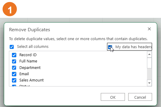
First decide what makes a record a duplicate. The recording selects the working range A1:K19, chooses Data > Remove Duplicates, and leaves My data has headers and Select all columns checked. At this point, source fields are in A:F and the helper columns G:K are still blank. Use the columns that define a duplicate in your own file; they determine the comparison key.

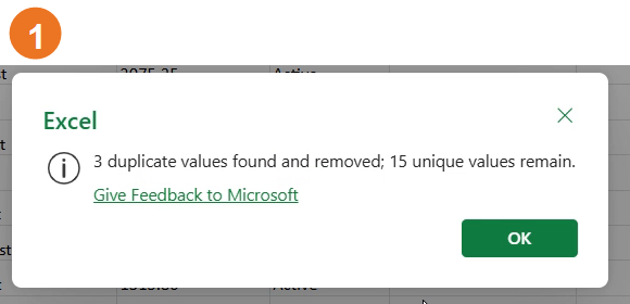
Excel for the Web Remove Duplicates dialog with the header option and Select all columns checked for the selected range; orange marker 1 highlights the settings. — Step 1. The recording keeps the header option on and all selected-range columns checked; helper columns are blank at this point.

Excel removes later matching rows from the selected range and keeps the first matching record. Here, the confirmation says three duplicates were removed and 15 unique records remain from the original 18. Check the count and spot-check the retained records.

Excel confirmation showing three duplicate values removed and 15 unique values remaining, marked with 1. — Result: three repeated records were removed; 15 remain. Removing duplicates changes the data, so work on a copy.

Excel removes the entire later row from the selected range, even when you use only some columns as the comparison key. For example, excluding an amount column can remove a row with a different amount if the checked fields match. Work on a copy and inspect the checked columns before confirming. Microsoft: filter for unique values or remove duplicates.

2. Clean extra spaces with TRIM

Extra leading, trailing, or repeated regular spaces can make text comparisons fail. In the sample, the source department is in column C. In the helper column G, enter this in G3 and fill down through the records:

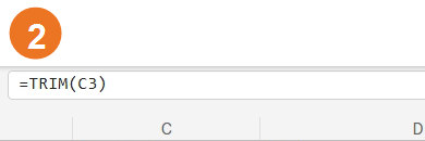
=TRIM(C3)

C3 is the source department for that row; the relative reference changes as you fill the formula down. In the capture, G is labeled Clean Department. Review the outputs before using them.

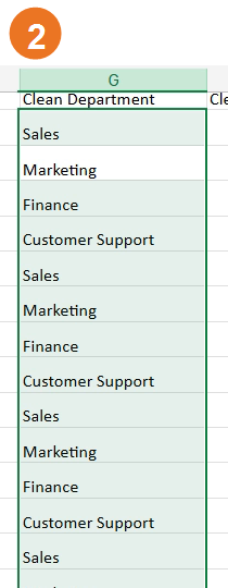
Close-up of Clean Department column G showing the cleaned values, marked 2. — Result: column G contains the trimmed department values.

To replace the original values, copy the reviewed helper results and paste them as values over the source cells, if that paste option is available in your current Web interface. Otherwise, keep the cleaned helper column and use it in later steps. TRIM handles ordinary spaces; some nonbreaking spaces copied from web pages need a separate cleanup.

Microsoft: TRIM function.

3. Standardize capitalization with PROPER

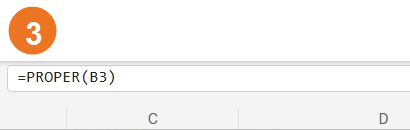
Names with all-uppercase, all-lowercase, or mixed capitalization are harder to scan. The sample name is in B3. In helper column H, enter this in H3 and fill down:

=PROPER(B3)

B3 is the original full name for that row; H3 is the corresponding cleaned result. PROPER capitalizes the first letter of each word and lowercases the remaining letters.

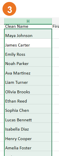
Clean Name column H showing corrected capitalization, marked 3. — Result: the name from B3 appears in cleaned case in column H.

Review names before replacing anything. PROPER can change intentional capitalization in names, abbreviations, and brand terms—for example, a name with an internal capital may need manual correction. Keep the original column until the cleaned results are checked. Microsoft: PROPER function.

4. Split names with Flash Fill

The demonstration’s Data ribbon exposes Flash Fill and shows it splitting the simple two-part names into First Name and Last Name columns. The source names are in column H; the outputs are in I and J. In this recorded Excel for the Web interface, the demonstrated command is Data > Flash Fill. Enter the first example for each output column if needed, select the remaining cells in that output column, then run Flash Fill and review the pattern it fills.

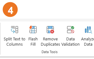
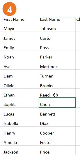
Close-up of the Data ribbon with the actual Flash Fill command highlighted, marked 4. — Recorded command: Data > Flash Fill.

First Name and Last Name output columns I and J with the demonstrated split, marked 4. — Result: the sample two-part names are separated into columns I and J.

Flash Fill availability can vary by Excel version and interface. Microsoft’s dedicated Flash Fill instructions list desktop Excel versions, while this captured Web interface visibly includes the command. If your Excel for the Web ribbon does not show Flash Fill, use a supported desktop Excel version or formulas for simple, consistently formatted names. For a name in B3 containing exactly one space, these formulas return the first word and the remaining text:

First part: =LEFT(B3,SEARCH(" ",B3)-1)
Remaining text: =TRIM(MID(B3,SEARCH(" ",B3)+1,LEN(B3)))

Those formulas are only a simple pattern example. Names may contain middle names, compound surnames, prefixes, suffixes, or no spaces; do not assume every name is just first plus last. Verify each split. Microsoft: using Flash Fill · Microsoft: split text into columns with functions.

5. Convert numbers stored as text with VALUE

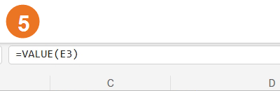
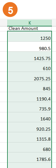
A number that looks numeric may be stored as text, so calculations or sorting can behave unexpectedly. In the sample, the source amount is in E3. In helper column K, enter this in K3 and fill down:

=VALUE(E3)

E3 is the text amount in the same row; K3 returns a numeric value. The formula bar in the screenshot shows the exact formula. The sample result is 980.5. Displayed decimal places depend on the cell’s number format.

Close-up of Clean Amount column K showing numeric results, marked 5. — Result: the helper column contains values Excel can use numerically. Confirm that the result matches the source amount.

Use VALUE only for quantities that should be numeric. Keep product codes, postal codes, and account identifiers as text when leading zeros matter.

VALUE depends on text that Excel recognizes as a number in your locale. Unrecognized symbols, separators, or malformed values can return an error. Review errors and totals. If you need to replace the source, copy reviewed results and paste as values where supported; otherwise retain the helper column. Microsoft: VALUE function.

6. Format the cleaned range as a table

After reviewing the cleaned columns you plan to keep, select a cell in that range and choose Home > Format as Table. In the dialog, confirm the range and check My table has headers when the first row contains field names. The recording formats A1:G16, a seven-column range containing one header row and 15 data rows. Your range will differ if you retain all helper columns.

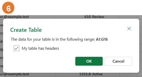
Format as Table dialog confirms range A1:G16 and the My table has headers option, marked 6. — Step 6. Check the detected range and header setting before applying a style.

Choose a readable style and confirm. The result is a table with filter controls in the headers and alternating row formatting. A table makes sorting and filtering easier; it does not guarantee the underlying data is correct.

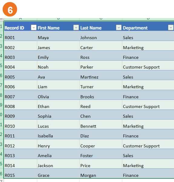
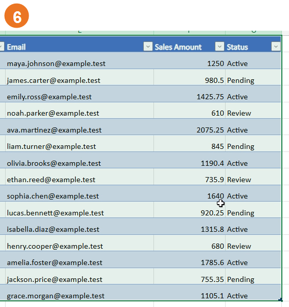
First half of the final formatted Excel table showing Record ID, First Name, Last Name, and Department columns, marked 6. — Final table, columns A–D: IDs, split names, and departments.

Second half of the final formatted Excel table showing Email, Sales Amount, and Status columns, marked 6. — Final table, columns E–G: email, numeric sales amount, and status.

Result: the recorded A1:G16 range is formatted as a table with 15 data rows. Recheck the range in your own workbook.

Microsoft: create and format tables.

Troubleshooting and limits

Remove Duplicates is unavailable or gives a surprising count: confirm you are editing the workbook, selected the intended range, and checked the correct headers and comparison columns. Undo immediately if the result is wrong, or reopen your untouched copy.
TRIM does not remove a visible gap: the character may be a nonbreaking space or another nonstandard character. Inspect the source and use a targeted cleanup method rather than replacing all spaces blindly.
PROPER changes a valid name or acronym: keep the original and correct those exceptions manually.
Flash Fill is missing or splits incorrectly: availability varies; check your Web ribbon, use a supported desktop version, or use the simple formulas above only when the text pattern is consistent. Review every output.
VALUE returns an error or an unexpected decimal: check currency symbols, separators, hidden characters, and regional number conventions. Compare the result with the original text.
The table omits rows or treats a header as data: reopen Format as Table and correct the range and header option.

Sources and optional video

Microsoft guidance: work with worksheet data in OneDrive; TRIM; PROPER; Flash Fill; VALUE; tables.

For more Excel guidance, visit The Click Test articles or the homepage.

Optional video walkthrough

Prefer to watch? This optional video covers the same six fixes using the fictional workbook, including the recorded Excel for the Web workflow. Open the walkthrough from this link, or follow the written steps and screenshots in this article: watch the Clean Messy Excel walkthrough.