

In the screenshots, orange outlines mark cells or controls to use or inspect. Key labels show which keys to press.
These six Excel for the Web shortcuts speed up common worksheet tasks: filling formulas, completing text patterns, adding totals, filtering a list, and turning a range into a table. This Windows walkthrough uses a fictional sales worksheet; follow the written steps without needing the video.
What you need
- A browser and Excel for the Web in editing mode. Microsoft offers free web apps with a Microsoft account; you can also use an eligible work or school account.
- A workbook you own or have permission to edit, stored in OneDrive or an organization’s SharePoint location. For practice, make a copy or use a blank workbook.
- A Windows keyboard for the exact key combinations shown. The source recordings show Excel for the Web on Windows, but the browser chrome is not visible, so the recording does not establish which browser was used.
No desktop Excel installation is needed for these web steps. The free and work or school experiences can differ by account and organization. See Microsoft’s free web apps overview and Excel for the web and OneDrive guide.
1. Fill Down — Ctrl+D
Use it for: copying the top cell’s contents and formula pattern down through a selected range.
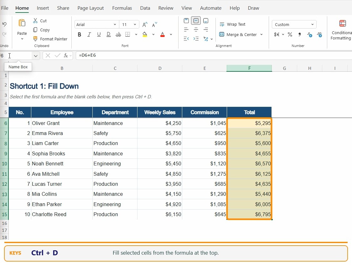
Selection: include the cell with the formula at the top and every destination cell below it. In this example, F6 already contains =D6+E6; select F6:F15.
- Enter or check the formula in the first cell, F6.
- Select F6 through F15. The top cell must contain what you want copied.
- Press Ctrl+D. Excel fills the selected cells and adjusts relative row references.
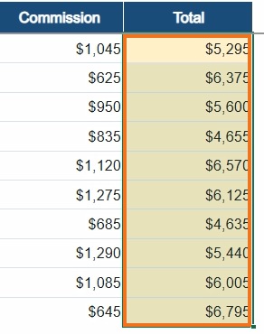
Result: F6:F15 displays each row’s weekly sales plus commission. Check the last row before using the totals.
2. Fill Right — Ctrl+R
Use it for: copying the leftmost cell’s formula across adjacent columns.
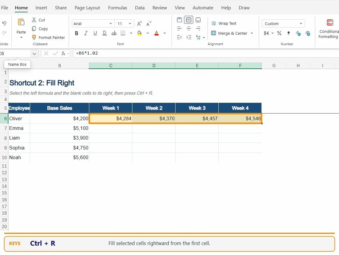
Selection: include the starting formula and the destination cells to its right. In the example, C6 contains =B6*1.02; select C6:F6.
- Enter the starting formula in C6.
- Select C6 through F6.
- Press Ctrl+R. Excel copies the formula across and adjusts the column references.
Result: the row shows four weekly sales values: $4,284, $4,370, $4,457, and $4,546.

=B6*1.02.
3. Flash Fill — Ctrl+E
Use it for: recognizing a text pattern, such as extracting first names from full names. Flash Fill writes fixed values, not live formulas.
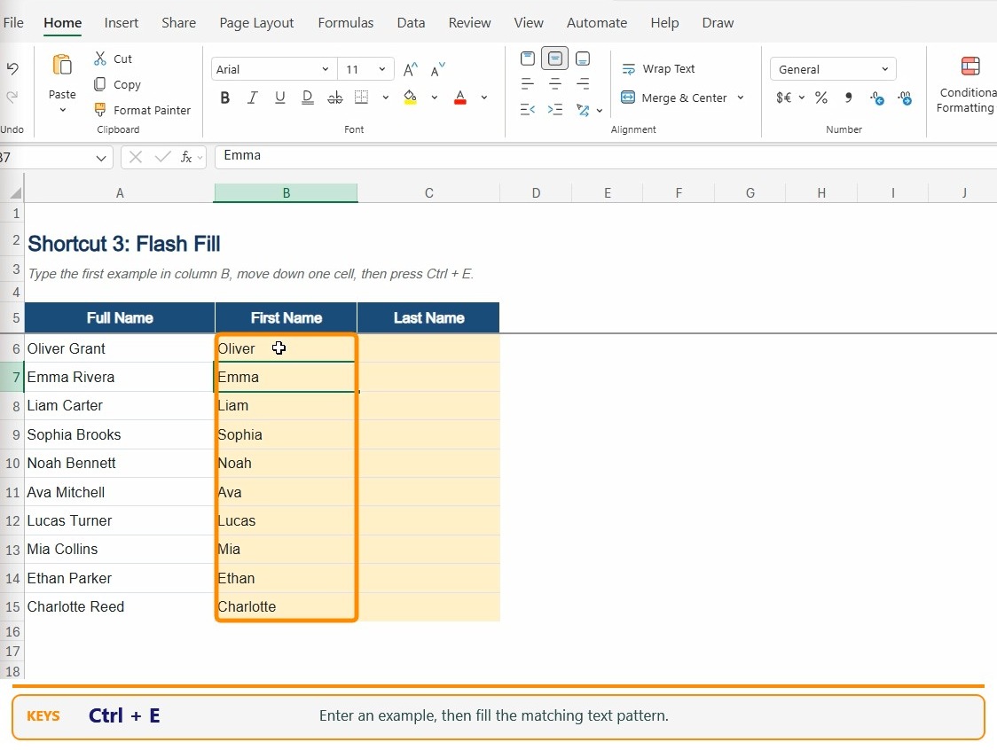
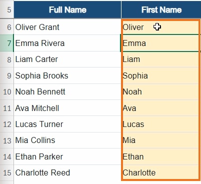
Selection: put the example in the adjacent output column. In the recording, full names are in A6:A15 and first names go in B6:B15.
- Type
Oliverin B6 besideOliver Grant. - Type
Emmain B7 besideEmma Rivera, then leave B7 active. - Press Ctrl+E. Excel detects the pattern and fills the remaining first names.
- Inspect several entries, especially unusual names, blanks, or compound names.
Result: the First Name column contains the matching first names. If the original names change, rerun Flash Fill or use a formula instead.
4. AutoSum — Alt+=
Use it for: inserting a SUM formula for a nearby run of numbers.
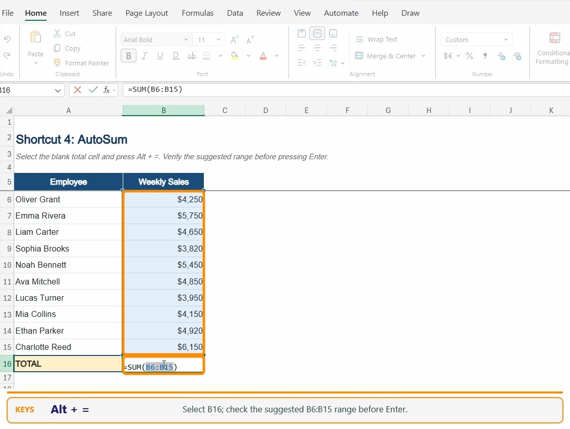
Selection: click the blank result cell below the values. In this example, choose B16 for the values in B6:B15.
- Select B16.
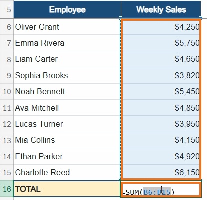
- Press Alt+=. Excel suggests
=SUM(B6:B15). - Check that the highlighted range contains exactly the values you intend to add. Edit the range if needed.
- Press Enter to calculate the total.
Result: the sample total is $47,940. That amount is the sum of the ten visible sales values. The available source capture ends with the suggested formula before Enter, so the screenshot shows the proposed range, not a committed result cell.
5. Toggle filters — Ctrl+Shift+L
Use it for: adding or removing filter controls on a plain data range.
Selection: click any cell inside a rectangular dataset with one header row. In this example, click inside the employee table.
- Click any data cell.
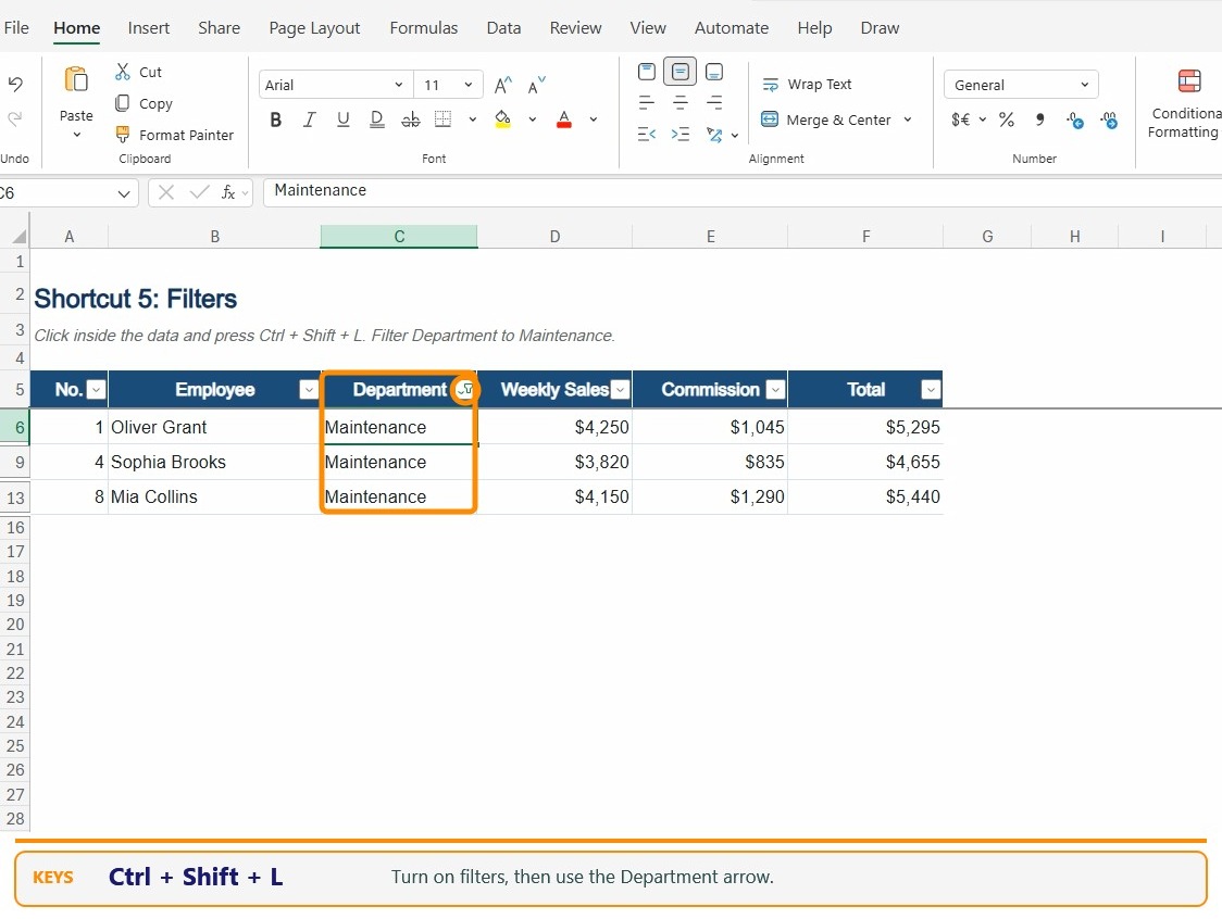
- Press Ctrl+Shift+L. Filter arrows appear in the header row.
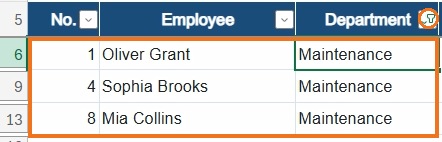
- To narrow the list, open the Department arrow, clear Select All, select Maintenance, and apply the filter.
- To show all rows again, clear the filter selection. Press the shortcut again only if you want to remove the filter controls.
Result: the example shows the three Maintenance records; other rows are hidden from view, not deleted.
6. Create a table — Ctrl+L
Use it for: converting a plain rectangular range into an Excel Table with header filter controls and table formatting.
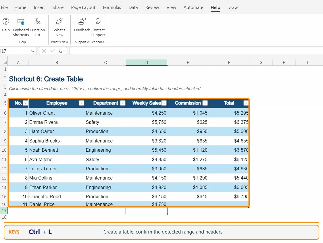
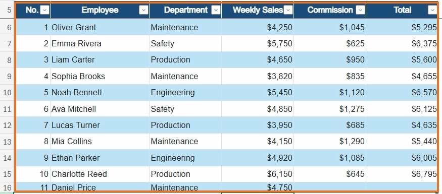
Selection: click a cell inside the data. Excel detects the surrounding range. The source example includes headers in row 5 and data through row 16.
- Click a cell inside the plain data range.
- Press Ctrl+L. Excel opens the Create Table dialog.
- Check that the proposed range is correct and that My table has headers is selected.
- Choose OK. Confirm the header filters and table styling appear.
Result: the data is a real Excel Table with header filter buttons and banded rows. If Ctrl+L opens the browser address bar, use Insert > Table or configure Excel’s browser shortcut override as described below.
Browser conflicts, Mac notes, and troubleshooting
Excel for the Web runs inside a browser, so a browser may capture a key before Excel receives it. For example, browsers commonly use Ctrl+L for the address bar, Ctrl+R to reload, and Ctrl+D for bookmarks; exact behavior varies by browser. Microsoft’s setting is at Help > Keyboard Shortcuts > Override browser shortcuts. Select the override option and review Show Overrides. If Ctrl+L is intercepted, choose Insert > Table. If Ctrl+R or Ctrl+D is intercepted, drag the starting cell’s fill handle across or down through the intended cells.
These steps use a Windows keyboard in Excel for the Web, not the desktop Excel app. Mac shortcuts can differ; open Help > Keyboard Shortcuts in your workbook to check the keys for your setup.
- Nothing happens: click a worksheet cell first and confirm you are editing the workbook, not typing into the formula bar or browser address bar.
- The wrong cells change: undo immediately, reselect the intended range, and retry on a copy.
- AutoSum suggests the wrong range: edit the range before pressing Enter.
- Flash Fill misses a pattern: add a clear example and review the output; it creates fixed values.
- Table range is wrong: edit the range and header setting in the Create Table dialog before choosing OK.
Watch the demonstration
The player is optional: all six procedures are written above. This is the related demonstration, 6 Excel Shortcuts That Save Time | Excel for the Web.
Open the video on YouTube if the embedded player does not load.
Official sources
- Microsoft: Keyboard shortcuts in Excel — includes Excel for the Web shortcuts and browser override guidance.
- Microsoft: keyboard shortcuts for tables — lists Ctrl+L as a table shortcut.
- Microsoft: Using Flash Fill — describes the Ctrl+E command and pattern examples.
- Microsoft: Add a list of numbers in a column — explains checking the proposed AutoSum range.
- Microsoft: free web apps and subscriptions — explains account access.
Related guides: The Click Test article library and The Click Test video library.